machine learning - 실습 2주차

machine learning

---

read_csv()

• 외부 text 파일, csv 파일을 불러와서 DataFrame으로 저장하는 방법

• Python의 pandas library

  에시

  data_path = join('.','dataset_for_lab02.csv')
  df = pds.read_csv(data_path)
  

  • 팁 : join을 이용하여 경로를 설정하면 환경에 영향을 받지않고 경로를 설정해줄수 있다.

    => data_path == '.\\dataset_for_lab02.csv'

  출처: https://rfriend.tistory.com/250 [R, Python 분석과 프로그래밍의 친구 (by R Friend)]

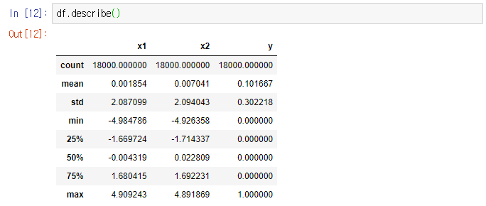
describe()

• 각정 통계향을 요약해서 출력해준다.
• 통계량은 series에 대해 요약이 수행된다.
• DataFrame의 경우 열에 대해 요약이 수행된다.

• 기본적으로 누락데이터(NaN)은 제외되고 데이터 요약이 수행되게 된다.

• https://kongdols-room.tistory.com/172

  

shape

• 행렬의 개수를 나타내준다.

• df.shape[0] : 행의 개수

• df.shape[1] : 열의 개수

plotly 라이브러리

• Plotly 라이브러리를 처음 사용한다면 설치가 필요하다.

  !pip install plotly
  

  을 주피터 노트북에서 실행하면 설치가 완료된다.

• plotly는 반응형, 오픈소스 그리고 브라우저 기반 시각화 라이브러리

데이터 시각화

##그림 생성
ax = go.Scatter(x=df.x1,y=df.x2,mode='markers')

## 여백 생성
fig=go.Figure()

## 여백에 그림 추가
fig.add_trace(ax)

## 여백의 속성 변경
fig_options={
    'layout' : dict(template='simple_white',
                   width=800, height=700,
                   title='Plotting toy example'),
}
fig.update(fig_options)

## 여백 시각화
fig.show()

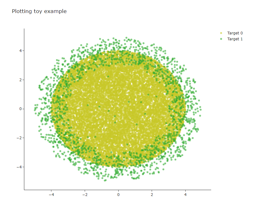
결과

## target == 0인 표본들의 그림 1 생성 / 노란색 마커
ax1 = go.Scatter(x=df.x1.loc[df.y==0],
                y=df.x2.loc[df.y==0],mode='markers',
                marker=dict(color='rgba(200,200,40,0.6)')
                 ,name='Target 0')
## target == 1인 표본들의 그림 2생성 / 초록색 마커
ax2 = go.Scatter(x=df.x1.loc[df.y==1],
                y=df.x2.loc[df.y==1],mode='markers',
                marker=dict(color='rgba(50,171,50,0.6)')
                 ,name='Target 1')

##여백 생성
fig=go.Figure()

## 그림 1,2를 여백에 추가
fig.add_trace(ax1)
fig.add_trace(ax2)

## 여백 속성 변경
fig_options={'layout':dict(template='simple_white',
                          width=800,height=700,
                          title='Plotting toy example'),}
fig.update(fig_options)

## 여백 시각화
fig.show()

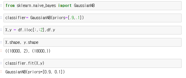
– 이제 위를 naive baesian 분류를 해볼것이다. [아래]

Naive Baesian classifier 실습

’

• 평가하기